Math Gamification
Instruction: please, use your google account

This test examines your ability to understand some basic definitions of game theory, such as players, moves, game types. You will play some rounds of Quatro Uno and Auction games and answer theoretical questions.
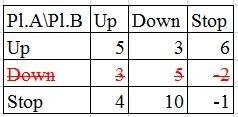
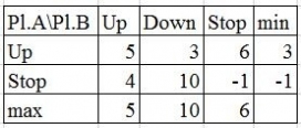
Test 2: Dominant and dominated strategies
Based upon a payoff matrix you shall eliminate dominated strategies.
Watch short videos and classify the situation: if it is a chicken game, a stag hunt dilemma or the battle of the sexes